Evaluating forecast models: train/test splits, time-series cross-validation and error metrics
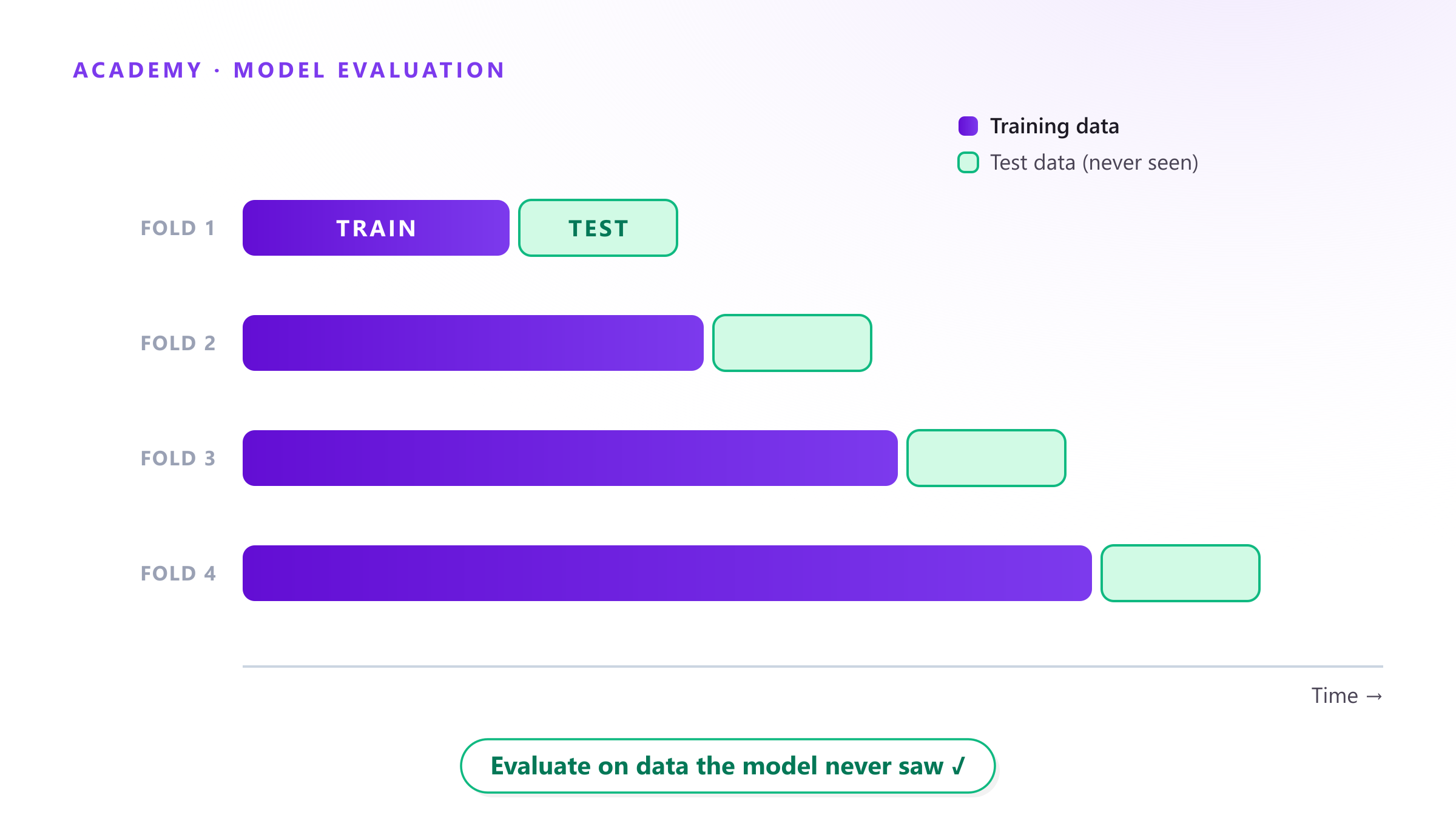
A model that fits its training history well tells you little about how it will forecast. Residuals are computed on data the model already saw, and flexible models can fit noise — so in-sample error systematically understates true forecast error (Hyndman & Athanasopoulos, FPP3 §5.8). Every claim about forecast accuracy should come from data the model never saw. This post covers the three tools that make that possible: the train/test split, time-series cross-validation, and the error metrics you compute on top.
Train/test split: temporal, never shuffled
For time series, the split is a cut in time: train on the past, test on the most recent segment. A test window of about 20% of the series is a common default, and it should be at least as long as the horizon you intend to forecast (FPP3 §5.8).
What you must not do is shuffle observations into random folds, as in standard k-fold cross-validation. Adjacent observations in a time series are correlated; shuffling puts the “future” inside the training set and leaks information. The exception is narrow: for purely autoregressive setups with uncorrelated errors, k-fold can remain valid (Bergmeir, Hyndman & Koo, 2018) — but for general pipelines with trend, seasonality or exogenous variables, keep the split temporal (Bergmeir & Benítez, 2012).
Rolling-origin cross-validation
A single split evaluates the model at one point in time. Rolling-origin evaluation — the time-series form of cross-validation — repeats it: train up to an origin, forecast the next window, advance the origin, repeat, and average the errors across folds (Tashman, 2000; FPP3 §5.10). The hero diagram above is exactly this: the training window expands, and the test block is always ahead of it.
You get a more robust error estimate, an error-vs-horizon curve, and protection against the lucky-split problem. In Python, sklearn.model_selection.TimeSeriesSplit implements the expanding-window scheme.
Which error metric, and when
All of these are computed on the test folds. They answer different questions (Hyndman & Koehler, 2006):
| Metric | Type | Strengths | Weaknesses |
|---|---|---|---|
| MAE | Scale-dependent | Robust, interpretable in units | Not comparable across series |
| RMSE | Scale-dependent | Penalizes large misses | Sensitive to outliers |
| MAPE | Percentage | Familiar to business users | Undefined at zero; penalizes over-forecasts more |
| sMAPE | Percentage | Bounded; used in M-competitions | Still unstable near zero |
| MASE | Scaled | Defined with zeros; comparable across series | Less intuitive to explain |
MASE scales the error by the in-sample MAE of a naive forecast, so MASE < 1 means “beats naive” on any series, including intermittent demand with zeros — the reason Hyndman & Koehler proposed it as the default for comparing across series. For aggregating error over a portfolio of SKUs in money-relevant terms, the business-side complement is WMAPE — covered in our metrics post.
Checklist
- Split temporally; test window ≥ forecast horizon.
- No leakage: scalers, feature encoders and hyperparameter tuning fit on train only.
- Use rolling-origin evaluation rather than one split when the series allows it.
- Report a scaled metric (MASE) alongside a business metric (WMAPE).
- Compare every model against a naive baseline — if it doesn’t beat naive out of sample, it isn’t adding value.
This is the evaluation discipline behind Forecast Studio: after each training, the app viewer shows the error metrics and lets you compare variables side by side, so the model you promote is the one that won on unseen data — you can reproduce everything in this post on the Free plan’s public tenant.
Sources: Hyndman & Athanasopoulos, Forecasting: Principles and Practice (3rd ed.), §5.8 & §5.10 · Hyndman & Koehler (2006), IJF · Tashman (2000), IJF · Bergmeir & Benítez (2012), Information Sciences · Bergmeir, Hyndman & Koo (2018), CSDA · scikit-learn TimeSeriesSplit