Stationarity in time series: unit-root tests, differencing and the Box-Cox transform
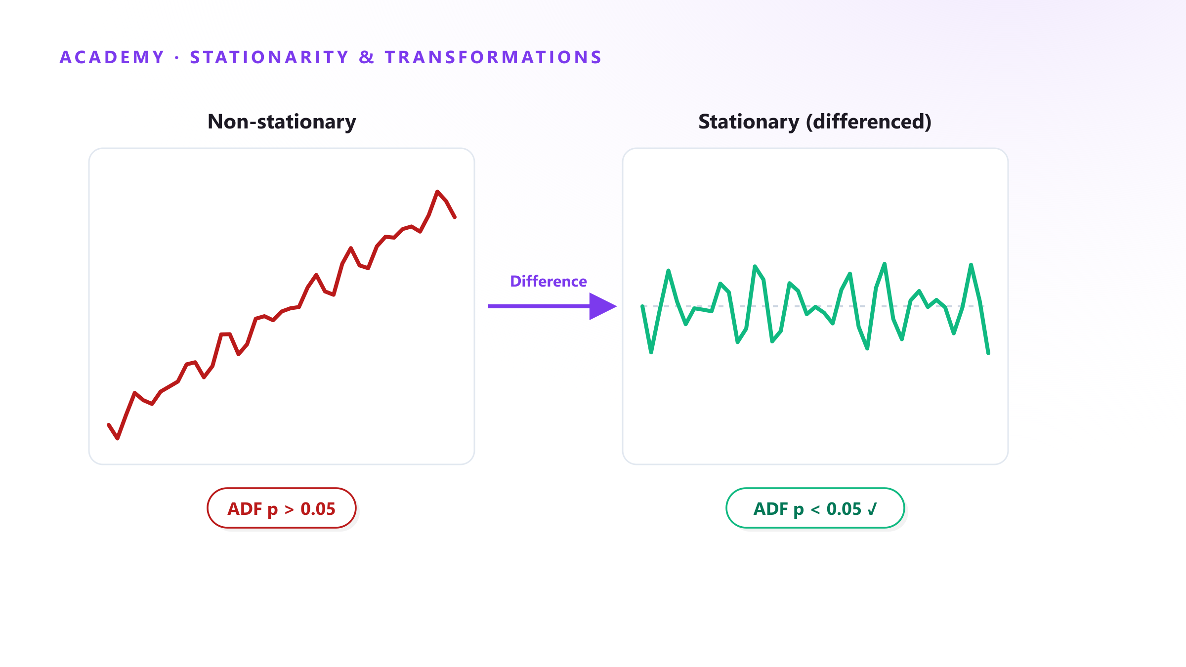
A time series is (weakly) stationary when its mean, variance and autocorrelation structure don’t change over time — no trend, no growing spread, no seasonal cycle (FPP3 §9.1). Stationarity matters because ARIMA’s AR and MA coefficients are only meaningful if the underlying process is stable enough for a fixed set of coefficients to describe it at every point in the series; fit ARIMA to a trending series without differencing it and the coefficients pick up spurious structure.
Testing for stationarity
Two complementary hypothesis tests are standard:
- Augmented Dickey-Fuller (ADF) — null hypothesis: the series has a unit root (is non-stationary). A low p-value (< 0.05) rejects it, evidence for stationarity (Dickey & Fuller, 1979).
- KPSS — null hypothesis is the opposite: the series is stationary. A low p-value here is evidence against stationarity (Kwiatkowski, Phillips, Schmidt & Shin, 1992).
Running both catches cases where one test’s assumptions don’t fit the data; agreement between them is stronger evidence than either alone.
Differencing: removing trend and seasonality
If the series fails the stationarity test, differencing — replacing yₜ with yₜ − yₜ₋₁ — typically removes a linear trend. One or two rounds of ordinary differencing is usually enough (over-differencing adds noise and unnecessary MA structure); a series with a seasonal cycle instead (or in addition) needs a seasonal difference, yₜ − yₜ₋ₘ, at the seasonal period m (FPP3 §9.1). This is exactly the d and seasonal D orders in ARIMA/SARIMA.
Variance stabilization: the Box-Cox transform
Differencing fixes a changing mean; it does nothing for variance that grows with the level (common in demand data — bigger volumes swing more in absolute terms). The Box-Cox transform applies a power transformation controlled by λ (λ=0 is the natural log; λ=1 shifts the series but leaves its shape unchanged) to stabilize variance before differencing. Guerrero (1993) proposed a method to pick λ automatically by minimizing the coefficient of variation of the seasonal sub-series — implemented as guerrero() in R’s fable and widely copied elsewhere.
Checklist
- Plot first: visible trend or growing variance is a strong hint before running any test.
- Run ADF and KPSS together; don’t rely on one test in isolation.
- Difference to fix the mean (trend, seasonality); Box-Cox/log-transform to fix the variance — apply the transform before differencing.
- Don’t over-difference: check the ACF of the differenced series for an unnecessarily large negative lag-1 autocorrelation, a common over-differencing symptom.
Forecast Studio’s pipeline runs these stationarity checks automatically before fitting statistical models, so the diagnostics behind this post are the same ones running under the hood — reproducible on the Free plan’s public tenant.
Sources: Hyndman & Athanasopoulos, FPP3 §9.1 · Dickey & Fuller (1979), JASA · Kwiatkowski, Phillips, Schmidt & Shin (1992), Journal of Econometrics · Box & Cox (1964), JRSS B · Guerrero (1993), Journal of Forecasting