ARIMA and SARIMA models: the Box-Jenkins method for time series forecasting

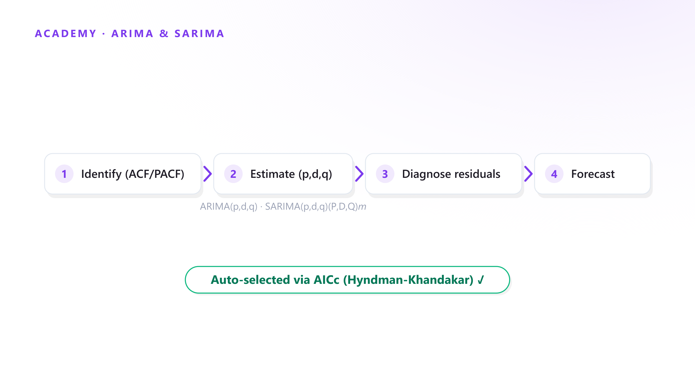
An ARIMA model forecasts a series from its own past — no external drivers, just the structure in the numbers themselves: how much a value depends on its recent history (autoregression), how much of a trend needs removing before that structure shows up (differencing), and how much of the noise carries forward (moving average). The method was formalized by Box & Jenkins (1970) and remains, more than 50 years later, one of the two standard baselines for univariate forecasting — in the M4 competition, all six pure machine-learning submissions underperformed the statistical Comb benchmark across its 100,000 series, and the winning method was a hybrid that combined exponential smoothing with a neural network (Makridakis, Spiliotis & Assimakopoulos, 2020).

The three components: AR, I, MA

ARIMA(p, d, q) combines:

• AR(p) — autoregression: the forecast is a linear combination of the last p observations.
• I(d) — integration: the series is differenced d times to remove trend before fitting.
• MA(q) — moving average: the forecast also depends on the last q forecast errors.

Fit the model to a series that isn’t stationary — mean and variance changing over time — and the AR/MA coefficients are unreliable (FPP3 §9.1); that’s why d comes first. See our post on stationarity and transformations for the tests and transforms that go into choosing it.

Seasonal series: SARIMA

Retail, e-commerce and most demand series carry a seasonal cycle a plain ARIMA can’t see. SARIMA(p,d,q)(P,D,Q)ₘ adds a second, seasonal set of AR/I/MA terms at lag m (12 for monthly data, 7 for daily-with-weekly pattern): a seasonal AR term correlates the value with the same period a year (or week) back, and seasonal differencing removes a repeating pattern the way plain differencing removes a trend (FPP3 §9.9).

Identifying the orders: ACF and PACF

Box & Jenkins’ original method reads the orders off two plots of a stationary series: the autocorrelation function (ACF) suggests q (an MA(q) process cuts off after lag q), the partial autocorrelation function (PACF) suggests p (an AR(p) process cuts off after lag p). In practice, most implementations now search a grid of (p,d,q) combinations and pick the one that minimizes AICc rather than reading plots by eye — the Hyndman-Khandakar algorithm (Hyndman & Khandakar, 2008) automates exactly this and ships as auto_arima in Python’s pmdarima and ARIMA() in R’s fable. statsmodels’ SARIMAX fits a given order and also accepts exogenous regressors (the “X” in SARIMAX) for holidays, promotions or price.

ARIMA vs. exponential smoothing

Both are standard univariate baselines and both are state-space models under the hood, but they start from different assumptions — and neither class is universally superior (FPP3 §9.10):

	ARIMA	ETS / Holt-Winters
Models	Autocorrelation in (differenced) errors	Level, trend, seasonality directly
Needs stationarity	Yes (via differencing)	No
Seasonal form	Multiplicative needs a log transform	Native additive or multiplicative
Typical use	Series with strong autocorrelation, engineering/econometric signals	Series with clear trend/seasonal structure, business demand

See our exponential smoothing post for the ETS side. Neither dominates universally — evaluate both out of sample with rolling-origin cross-validation and keep whichever wins.

Checklist

• Confirm stationarity (or difference until it holds) before fitting AR/MA terms.
• For seasonal data, use SARIMA or fit ETS instead — a plain ARIMA will miss the cycle.
• Prefer AICc-based automatic search (Hyndman-Khandakar) over hand-reading ACF/PACF for production pipelines.
• Always benchmark against a naive/seasonal-naive forecast and against ETS — report whichever wins on unseen data, not by assumption.

ARIMA and SARIMA are part of the model library Forecast Studio trains and compares automatically for every series — you can fit one on real data and see it side by side with ML alternatives on the Free plan’s public tenant.

Sources: Box & Jenkins, Time Series Analysis: Forecasting and Control (Wiley) · Hyndman & Athanasopoulos, FPP3 §9 · Hyndman & Khandakar (2008), JSS · Makridakis, Spiliotis & Assimakopoulos (2020), IJF — M4 Competition · statsmodels SARIMAX