Time series decomposition: separating trend, seasonality and the residual with STL
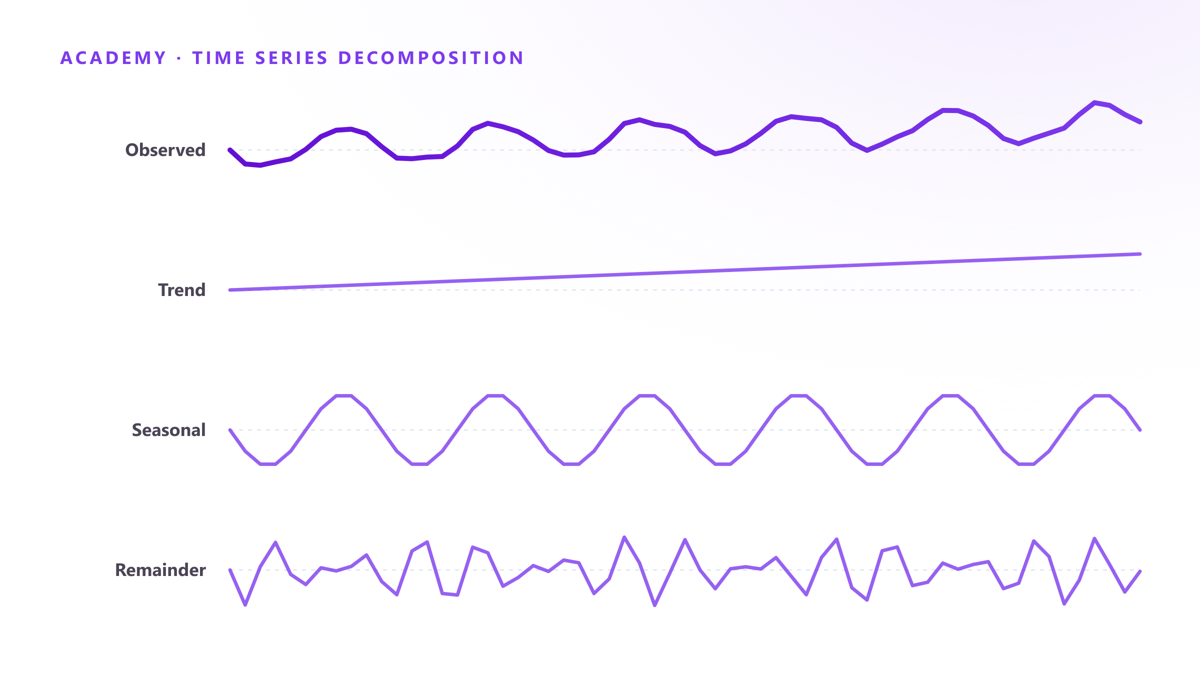
Before modeling a series, it helps to see what’s in it. Decomposition splits an observed series yₜ into a trend-cycle Tₜ, a seasonal component Sₜ and a remainder Rₜ — additively (yₜ = Tₜ + Sₜ + Rₜ) when seasonal swings stay roughly constant in size, multiplicatively (yₜ = Tₜ × Sₜ × Rₜ, or additive on the log scale) when they scale with the level (FPP3 §3.1).
Classical decomposition and its limits
The classical method estimates the trend with a moving average, then averages the detrended values by seasonal period. It’s simple and still common, but it has real weaknesses: the moving average leaves the first and last few observations without a trend estimate, it assumes the seasonal component is fixed over the whole series, and it isn’t robust to outliers, which leak straight into the remainder (FPP3 §3.4).
STL: Seasonal-Trend decomposition using Loess
Cleveland, Cleveland, McRae & Terpenning (1990) proposed STL to fix those issues. STL fits the trend and seasonal components with iterative Loess (locally weighted regression) smoothing, which means:
- The seasonal component can change over time — useful when a category’s peak season shifts.
- It handles any seasonal periodicity, not just monthly/quarterly.
- An optional robust mode down-weights outliers so they don’t distort the trend or seasonal estimate.
The trade-off is that STL only produces an additive decomposition — take logs first if the seasonal pattern is multiplicative. statsmodels’ STL and R’s fabletools::STL() implement it; the US Census Bureau’s X-13ARIMA-SEATS is the classical method’s production-grade successor, used for official statistics.
What decomposition is for
Decomposition isn’t itself a forecasting method (although a “seasonally naive” forecast can be built by extrapolating the trend and re-adding the last seasonal cycle). Its real value is diagnostic:
- Seeing the seasonal shape before choosing between ETS’s additive/multiplicative seasonality or an ARIMA seasonal order.
- Deseasonalizing a series before comparing it to a seasonally-blind metric or driver.
- Isolating the remainder to spot outliers or structural breaks that a raw plot hides under the seasonal swing.
Checklist
- Plot the series first — additive vs. multiplicative seasonality should be visible before you pick a method.
- Prefer STL over classical decomposition unless you specifically need X-13ARIMA-SEATS-style calendar adjustments.
- Use the robust STL option when the series has known outliers (promotions, stockouts, data errors).
- Treat decomposition as a diagnostic step, not a forecast — feed what you learn into ETS, SARIMA or an ML model, then validate out of sample.
Forecast Studio’s model viewer plots the trend and seasonal components it fits behind every forecast, so you can sanity-check the shape before trusting the number — try it on the Free plan’s public tenant.
Sources: Hyndman & Athanasopoulos, FPP3 §3 · Cleveland, Cleveland, McRae & Terpenning (1990), STL · statsmodels STL · U.S. Census Bureau, X-13ARIMA-SEATS