Exponential smoothing and ETS models: from simple smoothing to Holt-Winters
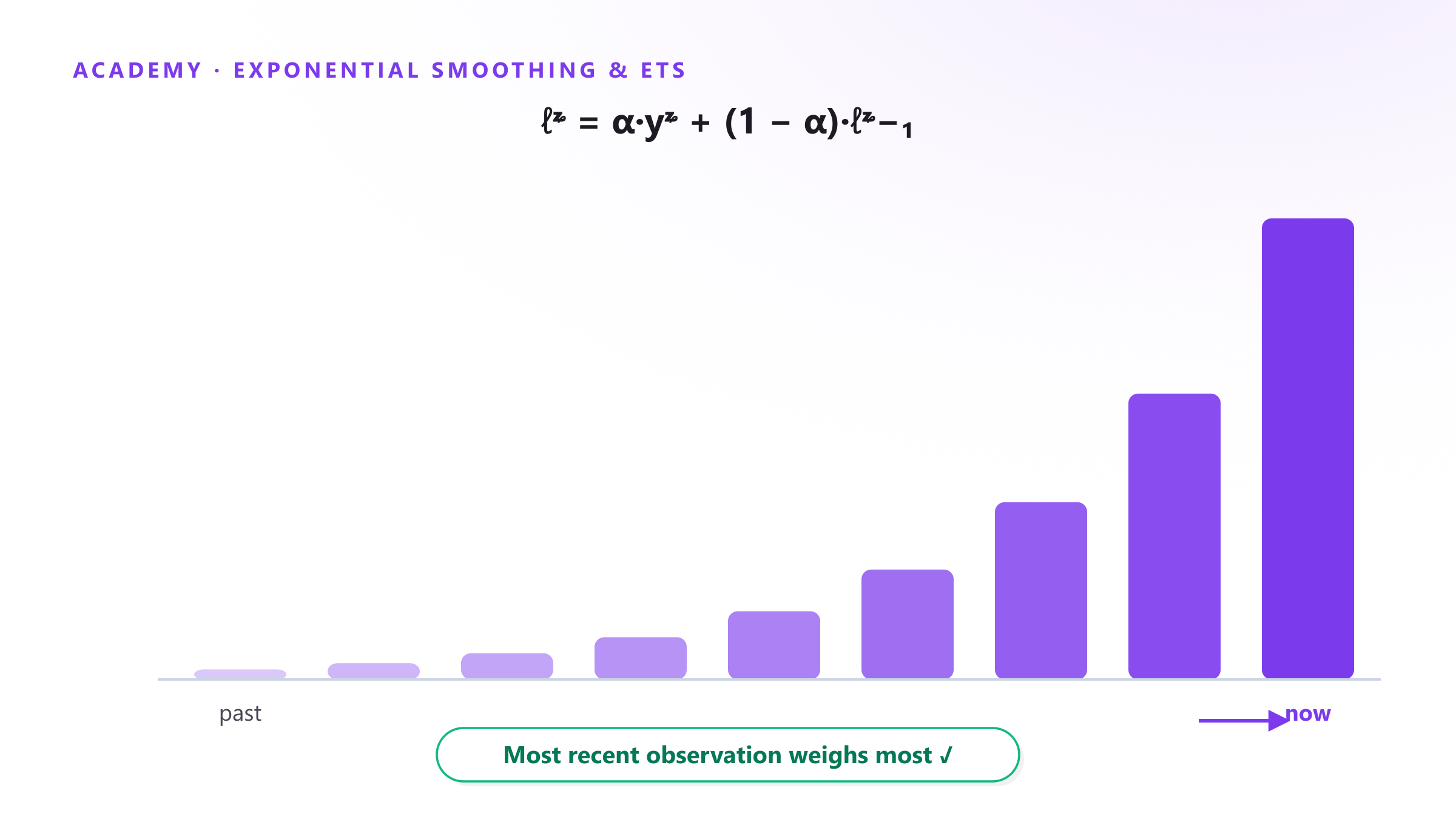
Exponential smoothing forecasts the next value as a weighted average of the past, but the weights decay exponentially instead of dropping off a sharp cutoff — the most recent observation matters most, older ones matter less and less but never zero (FPP3 §8.1). Winters (1960) extended the method with trend and seasonal components, and the resulting family — simple, Holt’s, Holt-Winters — is, alongside ARIMA, one of the two standard baselines every forecasting evaluation is measured against.
Simple exponential smoothing
For a series with no trend or seasonality, the level update is:
ℓₜ = α·yₜ + (1 − α)·ℓₜ₋₁
with 0 < α < 1. A high α reacts fast to recent changes (and to noise); a low α smooths harder. In practice α is fit by minimizing the sum of squared one-step errors, not chosen by hand.
Adding trend and seasonality: Holt-Winters
Holt (1957) added a trend component (a second smoothed series tracking the slope); Winters (1960) added a seasonal component on top, giving Holt-Winters two forms:
- Additive — seasonal swings of roughly constant size regardless of the level.
- Multiplicative — seasonal swings that scale with the level (a bigger baseline means a bigger seasonal bump in absolute terms) — the common case for demand data with strong growth.
ETS: the state-space framework
ETS stands for Error, Trend, Seasonal — each with none/additive/multiplicative options, giving up to 30 model variants (Hyndman, Koehler, Snyder & Grose, 2002). Framing exponential smoothing as a state-space model gives it something the classical formulas didn’t have on their own: a proper likelihood, which means AICc-based automatic model selection and analytically derived prediction intervals rather than only point forecasts (Hyndman & Athanasopoulos, FPP3 §8.8). statsmodels’ ETSModel and R’s fable::ETS() both implement this and pick the best variant automatically.
When ETS over ARIMA
Both are legitimate defaults: neither class is universally superior (FPP3 §9.10), and Gardner’s review of five decades of empirical evidence finds exponential smoothing remarkably robust in practice, including across the M-competitions (Gardner, 2006). ETS tends to be the simpler first attempt on series with a visually clear trend/seasonal shape and no need to model autocorrelated errors directly; it also requires no stationarity pre-processing, unlike ARIMA. It’s a reasonable default baseline before reaching for anything more complex.
Checklist
- Start simple: no trend/seasonal component beats a needless one — check both against a seasonal-naive baseline.
- Let software select additive vs. multiplicative seasonality (and the smoothing parameters) via AICc, not by eye.
- ETS gives closed-form prediction intervals — always report them alongside the point forecast (see our post on prediction intervals).
- Compare against ARIMA and against your production model out of sample (rolling-origin CV) before picking a winner.
ETS is one of the baselines Forecast Studio benchmarks every trained model against, so you can see exactly how much a more complex model is (or isn’t) buying you — reproducible on the Free plan’s public tenant.
Sources: Hyndman & Athanasopoulos, FPP3 §8 · Winters (1960), Management Science · Hyndman, Koehler, Snyder & Grose (2002), IJF · Gardner (2006), IJF · statsmodels ETSModel