Treating every SKU the same is the most expensive default in planning. A planner with 3,000 products and a same-effort policy gives the item that funds the payroll exactly as much attention as the one that sells twice a year. ABC/XYZ analysis is the classic two-axis fix: rank your catalog by value (ABC) and by demand variability (XYZ), cross the two, and you get nine cells with a clear strategy each. You can build the first version from a sales export in an afternoon — and it shows you precisely where a better forecast pays off most.

ABC: the value axis

The idea is the Pareto principle — the famous 80/20 rule — put to work on inventory. H. Ford Dickie, an engineer at General Electric, formalized it in 1951 in ABC Inventory Analysis Shoots for Dollars, Not Pennies: focus management attention where the money is, not where the part count is.

The mechanics take three steps:

Annual consumption value per SKU = units sold × unit cost (or revenue, or margin — pick the measure your business actually optimizes).
Sort descending and accumulate the share of total value.
Cut into classes. The common convention: A = the SKUs covering the top ~80% of value (typically only ~20% of items), B = the next ~15%, C = the last ~5% of value spread across roughly half the catalog.

The cut-offs are conventions, not laws — what matters is that the classes get different treatment. One pitfall up front: ranking by units instead of value silently promotes cheap fast-movers into A and demotes the products that actually carry your margin.

XYZ: the variability axis

ABC says nothing about how hard a product is to plan. That is the second axis: classify each SKU by the coefficient of variation (CV) of its demand over the last 12+ months:

CV = σ(demand) ÷ mean(demand)

The cut-offs used in practice (AbcSupplyChain, Mecalux):

Class	CV	Demand pattern
X	< 0.5	stable, predictable
Y	0.5 – 1.0	fluctuating — trend, seasonality
Z	> 1.0	erratic or intermittent

One honest nuance before you take raw CV at face value: a strongly seasonal product looks like Z on raw demand — big swings, high σ — yet is perfectly predictable to a model that understands the calendar. The demand-categorization literature (Syntetos, Boylan & Croston) splits demand patterns precisely because the right forecasting method differs by pattern. So once you have a real forecast, reclassify on the CV of your forecast error instead of raw demand — the same σ that should drive your safety stock. Variability you can predict is not risk; it is just shape.

The matrix: nine cells, nine strategies

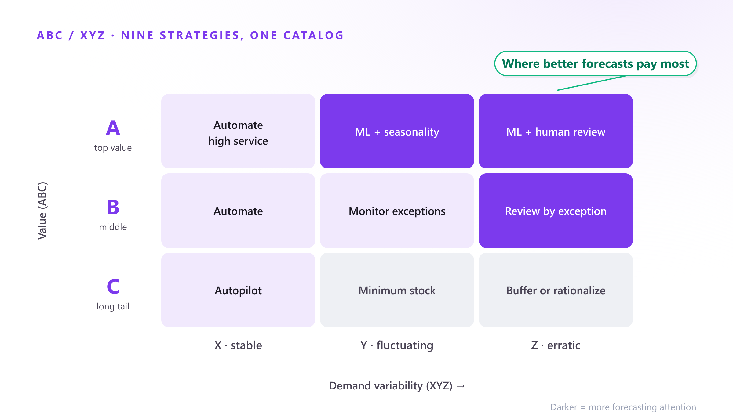
Cross the two axes and the planning policy almost writes itself:

	X — stable	Y — fluctuating	Z — erratic
A — top value	Automate the forecast, high service level, lean buffer	ML forecast with seasonality and promotions, monthly review	ML forecast plus human review — your hardest, most valuable fight
B — middle	Automate, touch rarely	Automate, monitor exceptions	Review by exception, moderate buffer
C — long tail	Full autopilot, simple reorder point	Autopilot with a minimum stock	Question the SKU: make-to-order, rationalize or a deliberately cheap buffer

Read it as an effort map: the upper-right is where forecasting attention concentrates (high value, hard demand), the lower-left is where automation should run untouched, and CZ is where the honest conversation is about the product, not the forecast.

A worked example

Monthly demand for three SKUs over the last year:

	Mean	σ	CV	Class
SKU 1	1,000	120	0.12	X
SKU 2	400	280	0.70	Y
SKU 3	60	90	1.50	Z

Now add the value axis: if SKU 1 is also an A by revenue, it is an AX — automate it, give it a 98% service level, and spend the time you saved on the AZ items, where every point of forecast accuracy converts directly into fewer stockouts and less buffer.

Differentiated service levels — the payoff

The matrix earns its keep when it drives policy. Setting one global service level over-protects half the catalog and under-protects the other half — which is why ASCM recommends setting service levels per product group, not globally. High service (and the Z factor that comes with it) on the A row; leaner targets on the tail. And because safety stock scales linearly with forecast error, every error point you remove on the A row frees working capital where it is most concentrated.

Your accuracy metric should think the same way: WMAPE weights error by volume, so it is effectively an ABC-aware metric — it already cares most about the SKUs your matrix calls A.

Pitfalls to avoid

A static matrix. Products migrate — launches start as Z, mature into X, decline back. Re-run the classification quarterly.
One single criterion. A $2 component that stops a production line is a C by value and critical by consequence. Keep a manual “critical” flag alongside the matrix.
Reading CZ as “ignore”. It means decide deliberately — make-to-order, rationalize, or hold a cheap buffer — not “stop looking”.
Classifying on raw CV forever. As your forecast improves, the honest variability axis is forecast error, not raw demand (see above).

Where the forecast fits

Be careful with the wrong conclusion: the matrix is not a license to forecast less. It is a map of where each point of forecast accuracy pays the most — and the answer is the A row and the Y/Z columns. Stable X items are cheap to automate; the erratic, valuable ones are exactly where Machine Learning with exogenous variables out-forecasts manual methods — seasonality, promotions and calendar effects are what turn an apparent Z into a planned Y. A better model literally moves SKUs toward the easy side of your matrix.

That is what Forecast Studio does nightly across the whole catalog: a fresh statistical forecast per SKU, global models that give even short-history products a usable baseline, and the error measured so your matrix stays honest.

Want to see your own catalog on this matrix? Book a free demo and we’ll segment it with you in 30 minutes.

Sources: Dickie, ABC Inventory Analysis Shoots for Dollars, Not Pennies (Factory Management and Maintenance, 1951) · Juran, Guide to the Pareto Principle · AbcSupplyChain, ABC XYZ Analysis · Mecalux, ABC XYZ analysis: pros and cons · Syntetos, Boylan & Croston, On the categorization of demand patterns, JORS · ASCM, Safety stock: a contingency plan

ABC/XYZ analysis: stop treating every SKU the same