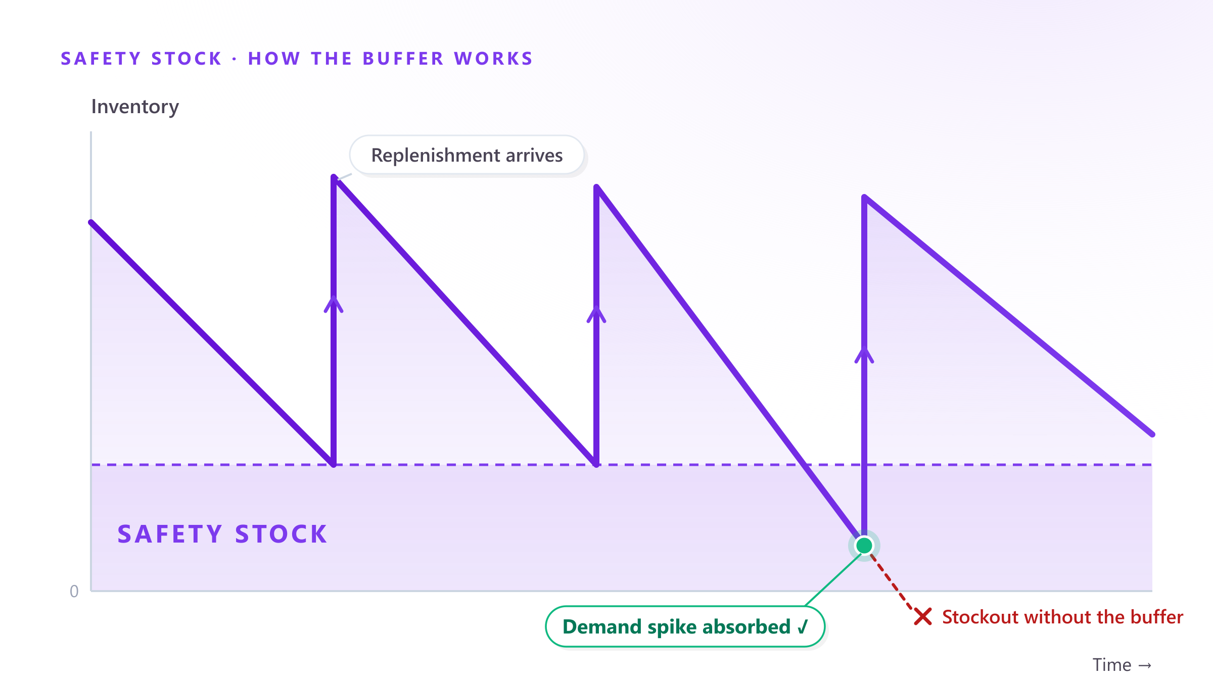
Safety stock is the extra inventory you hold to absorb the difference between what you forecast and what actually happens. It is the cushion that keeps you selling when demand spikes or a supplier ships late.

The stakes on both sides are well documented. A Harvard Business Review study by Corsten and Gruen put the cost of stockouts at about 4% of annual sales for a typical retailer — and found that nearly a third of shoppers facing an empty shelf simply buy the item from a competitor. Hold too much, though, and the carrying cost of inventory — capital, storage, insurance, obsolescence — typically runs 15–25% of its value per year. Safety stock is the dial between those two losses, so it deserves better than a guess.

Why a fixed “weeks of cover” rule fails

Many teams set safety stock as a flat rule — “always keep three weeks.” The problem is that not every product behaves the same. A stable, high-volume SKU barely needs a buffer, while an erratic one can swing wildly week to week. Applying the same rule to both over-stocks the easy items and under-stocks the risky ones — capital parked where there is no risk, stockouts where there is.

Size it from variability and lead time

A better starting point ties the buffer to two things you can measure:

Demand variability — how much real demand bounces around the forecast.
Lead time — how long replenishment takes, and how reliable it is.

The classic formula scales a service-level factor (Z) by the standard deviation of demand over the replenishment lead time:

Safety stock = Z × σ(demand) × √(lead time)

Z comes straight from the normal distribution and encodes the service level you want to protect — the share of replenishment cycles you get through without a stockout:

Service level	Z factor
90%	1.28
95%	1.64
98%	2.05
99%	2.33
99.9%	3.09

One subtlety the textbooks gloss over: if you forecast, the σ that belongs in the formula is the standard deviation of your forecast error, not of raw demand. What you are buffering against is what your forecast misses — predictable seasonality shouldn’t inflate the buffer.

A worked example

Say a SKU sells 100 units per week on average, the weekly demand variability is σ = 30 units, and your supplier reliably delivers in 4 weeks. For a 95% service level:

SS = 1.64 × 30 × √4 = 98 units — about one week of demand.

Want 99% instead? Swap in Z = 2.33 and the buffer jumps to 140 units. Same product, same supplier — the only thing that changed is how much risk you chose to cover.

When the lead time varies too

Real suppliers are not metronomes, and lead time variability is often the bigger risk. The extended formula — popularized by Peter King in APICS Magazine — adds a term for it:

SS = Z × √( LT × σ²demand + σ²LT × D² )

Take the same SKU, but now the supplier’s 4-week lead time swings by ±1 week (σLT = 1). At 95% service:

SS = 1.64 × √(4 × 30² + 1² × 100²) = 1.64 × √13,600 ≈ 191 units

Nearly double the buffer — and the demand numbers didn’t change at all. One unreliable supplier can cost you more inventory than all your demand noise combined, which is why supplier lead times deserve the same measurement discipline as sales.

The service-level trap

Notice how Z grows: moving from 95% to 99% inflates the buffer by 42%, and chasing 99.9% nearly doubles it. Protection gets exponentially more expensive as you approach 100% — which is why ASCM notes that typical service-level goals sit in the 90–98% range and recommends setting Z per product group, not globally: high service on the A items that drive your revenue, leaner buffers on the long tail.

Forecast quality changes everything

Here is the part teams miss: the buffer scales linearly with forecast error. Cut the error in half and you need half the safety stock for the same service level. McKinsey estimates that AI-driven forecasting reduces forecast errors by 20–50% — which translates directly into 20–50% less buffer across the catalog, working capital quietly freed without touching service.

That is the logic behind pairing demand planning with Machine Learning with per-SKU inventory math: Forecast Studio recomputes forecasts nightly, so your buffers can follow reality instead of last quarter’s spreadsheet. And before you trust any number, measure your current error with WAPE or MAPE — you can’t size a buffer against an error you haven’t quantified.

Conclusion

Safety stock is not a number you set once. It is a per-SKU, formula-driven quantity that should flex as demand patterns, forecast accuracy and supplier reliability shift. Get it right and you stop paying twice — once in lost sales, once in frozen capital.

Want to see what your buffers look like with your own data? Book a free demo and we’ll show you Forecast Studio in action in 30 minutes.

Sources: Corsten & Gruen, Stock-Outs Cause Walkouts, HBR · King, Crack the Code: Understanding safety stock, APICS Magazine · ASCM on safety stock and service levels · NetSuite, inventory carrying costs · McKinsey, AI-driven operations forecasting

Safety stock, explained: how much buffer inventory do you really need